Henk's tech blog

a weblog about IT optimization

Recently, with some colleagues, I was working on a project with a serious challenge; there was this Analysis Server 2012 system with 40 physical cores, half a Terabyte of RAM and 10TB of SSD storage waiting to get pushed to its limits but it was installed via the famous ‘next,next finish’ setup approach and we had to tune the box from scratch. Also we had to pull the data from a database running on another box which means the data processing will be impacted by the network round-tripping overhead. 

With a few simple but effective tricks for tuning the basics and a methodology on how to check upon the effective workload processed by Analysis Server you will see there’s a lot to gain! If you take the time to optimize the basic throughput, your cubes will process faster and I’m sure, one day, your end-users will be thankful! This Part 1 is about tuning just the processing of a single partition.

Quantifying a baseline

So, where to start? Well to quantify the effective processing throughput, just looking at Windows Task Manager and check if the CPU’s run at 100% full load isn’t enough; the metric that works best for me is the ‘Rows read/sec’ counter that you can find in the Windows Performance monitor MSOLAP Processing object. 

Just for fun… looking back in history, the first SSAS 2000 cube I ever processed was capable of handling 75.000 Rows read/sec, but that was before partitioning was introduced; 8 years ago, on a 64 CPU Unisys ES7000 server with SQL- and SSAS 2005 running side by side I managed to process many partitions in parallel and effective process 5+ Million Rows reads/sec (== 85K Rows read/sec per core).

 

Establishing a baseline – Process a single Partition

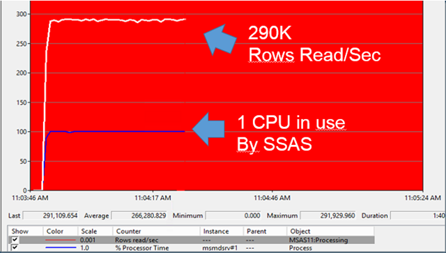
Today, with SSAS 2012 your server should be able to process much more data; if you run SQL and SSAS side by side on a server or on your laptop you will be surprise on how fast you can process a single partition;  expect 250-450K Rows read/sec while maxing out a single CPU at 100%.

As an impression of processing a single partition on a server running SSAS 2012 and SQL 2012 side by side using the SQL Server Native Client:  the % processor time of the SSAS process (MSMDSRV.exe) is at 100% flatline. Does this mean we reached maximum processing capacity? Well… no!  There is an area where we will find a lot of quick wins;  lets try if we can move data from A (the SQL Server) to B (the Analysis Server) faster.

100% CPU?

Max’ing out with a flatline on a 100% load == a single CPU may look like we are limited by a hardware bottleneck. But just to be sure lets profile for a minute where we really spend our CPU ticks. My favorite tool for a quick & dirty check is Kernrate (or Xperf if you prefer).

Command line:

Kernrate -s 60 -w -v 0 -i 80000 -z sqlncli11 -z msmdsrv -nv msmdsrv.exe -a -x -j c:\symbols;

Surprisingly more than half of our time isn’t spend in Analysis Server (or SQL server) at all, but in the SQL native Client data provider! Lets see what we can do to improve this.

 

Quick Wins

1) Tune the Bios settings & Operating system

Quick wins come sometimes from something that you may overlook completely, like checking the BIOS settings of the server. There is a lot to gain there; expect 30% improvement -or more-  if you disable a couple of energy saving options. (its up to you to revert them and save the planet when testing is done…)

For example: 

– Enter the Bios Power options menu and see if you can disable settings like ‘Processor Power Idle state’. 

– In the Windows Control Panel, set the Server Power Plan to max. throughput (up to Windows 2008R2 this is like pressing the turbo switch but on Windows 2012 the effect is marginal but still worth it).

 

2) Testing multiple data providers

Like the kernrate profiling shows, a lot of time is spend in the network stack for reading the data from the source. This applies to both side by side (local) processing as well as when you pull the data in over the network.

Since the data provider has a significant impact on how fast SSAS can consume incoming data, lets check for a moment what other choices we have available; just double click on the cube Data Source

 

Switching from the SQL Native Client to the Native OLE DB\ Microsoft OLE DB Provider for SQL Server brings the best result: 32% higher throughput!

 

SSAS is still using a single CPU to process a single partition but the overall throughput is significant higher when using the OLE DB Provider for SQL Server:

 

To summarize; with just a couple of changes the overall throughput per core just doubled!

 

Reading source data from a remote Server faster

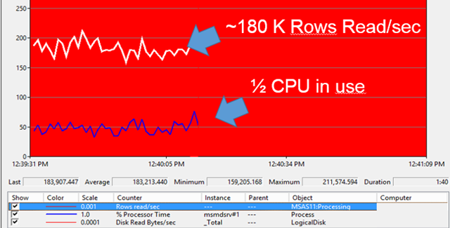
if you run SSAS on a separate server and you have to pull all the data from a database running on another box, expect the base throughput to be significant less due to processing on the network stack and round tripping overhead. The tricks that apply to the side by side processing also apply in this scenario:

1) Process the Partition processing baseline against the remote server.

Less rows are processed when reading from a remote server (see fig.); also the MSMDSRV process is effective utilizing only 1/2 of a CPU. The impact of transporting the data from A to B over the network is significant and worth optimize. Lets focus our efforts on optimizing this first. 

 

2)  Increase the network Packet Size from 4096 bytes  to 32 Kbyte.

Get more work done with each network packet send over the wire by increasing the packet size from 4096 to 32767;  this property can be set via the Data Source – Connection String too; just select on the left ‘All’  and scroll down till you see the ‘Packet Size’ field.

The throughput gain is significant:

 

Summary

When you have a lot of data to process with your SQL Server Analysis Server cubes, every second you spend less in updating and processing may count for your end-users; by monitoring the throughput while processing a single partition from a Measure Group you can set the foundation for further optimizations. With the tips described above the effective processing capacity on a standard server more  than doubled. Every performance gain achieved in the basis will pay back later while processing multiple partitions in parallel and helps you to provide information faster! 

In part II we will zoom into optimizing the processing of multiple partitions in parallel.