Special thanks to Dirk Gubbels for his contribution on the data type optimization part and review!(Follow Dirk on Twitter: @QualityQueries).
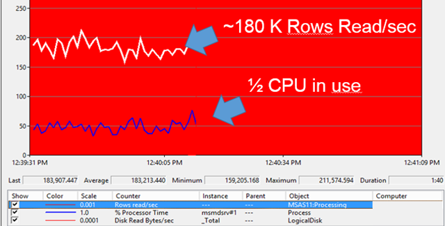
In part 1 we looked at a method to quantify the work that gets done by SQL Server Analysis Server and found that the OLE DB provider with a network packet size of 32767 brings best throughput while processing a single partition and maxing out the contribution per single CPU.
In this 2nd part we will focus on how to leverage 10 cores or more (64!) and benefit from every of these CPU’s available in your server while processing multiple partitions in parallel; hope the tips and approach will help you to test and determine the maximum processing capacity of the cubes on your SSAS server and process them as fast as possible!
Quick Wins
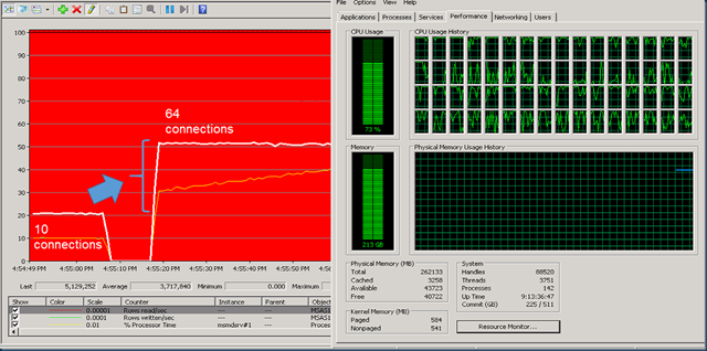
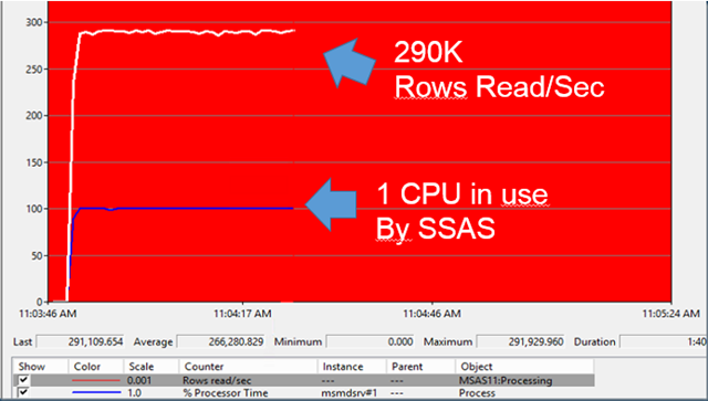
If you have more than 10 cores in your SSAS server the first thing you’ll notice when you start processing multiple partitions in parallel is that Windows performance counter ‘% Processor time’ of the msmdsrv process is steady at 1000% which means 10 full CPU’s are 100% busy processing. Also the ‘Rows read/sec’ counter will top and produce a steady flat line similar to the one below at 2 million Rows read/sec (==200K rows read/sec per CPU):

In our search for maximum processing performance we will increase the number to reflect the # Cores by modifying the Data Source Properties. Change the ‘Maximum number of connection’ from 10 into the # Cores in your server. In our test server we have 32 logical- and 32 Hyperthreaded = 64 cores available.
1) # Connections
By default each cube will open up a maximum of 10 connections to a data source. This means that up to 10 partitions are processed at the same time. See picture below: 10x status ‘In Progress- ’ for the AdventureWorks cubes which is slightly enpanded to span multiple years:

Just by changing the number of connections to 64 the processing of 64 partitions in parallel results in an average throughput of over 5 million Rows read/sec, utilizing 40 cores (yellow line)
This seems a great number already but its effective (5 million rows/40 cores =) 125K Rows per core and we do still see a flat line when looking at the effective throughput; this tells us that we are hitting the next bottleneck. Also the CPU usage as visible in Windows Task Manager isn’t at its full capacity yet!

Time to fire up another Xperf or Kernrate session to dig a bit deeper and zoom into the CPU ticks that are spend by the data provider:
Command syntax:
Kernrate -s 60 -w -v 0 -i 80000 -z sqlncli11 -z msmdsrv -z oleaut32 -z sqloledb -nv msmdsrv.exe -a -x -j c:\websymbols > SSAS_trace.txt

This shows an almost identical result as the profiling of a single partition in blog part I.
By profiling around a bit and checking on both the OLEDB and also some SQL native client sessions surprisingly you will find that most of the CPU ticks are spend on… data type conversions.

The other steps make sense and include lots of data validation; like, while it fetches new rows it checks for invalid characters etc. before the data gets pushed into an AS buffer. But the number 1 CPU consumer, CDataSource::DataConvert is an area that we can optimize!
(To download a local copy of the symbol files yourselves, just install the Windows Debugger by searching the net for ‘windbg download’ and run the symchk.exe utility to download all symbols that belong to all resident processes into the folder c:\websymbols\;
C:\Program Files (x86)\Windows Kits\8.1\Debuggers\x64\symchk.exe /r /ip * /s SRV*c:\websymbols\*http://msdl.microsoft.com/download/symbols )
2) Eliminate Data type conversions
This is an important topic; if the data types between your data source and the cube don’t match the transport driver will need a lot of time to do the conversions and this affects the overall processing capacity; Basically Analysis Server has to wait for the conversion to complete before it can process the new incoming data and this should be avoided.
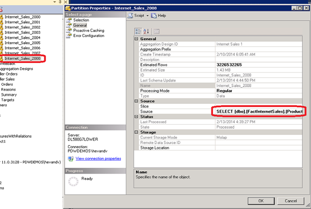
Let’s go over an AdventureWorksDW2012 Internet_sales partition as example:

By looking at the table or query that is the source for the partition, we can determine it uses a range from the FactInternetSales table. But what data types are defined under the hood?
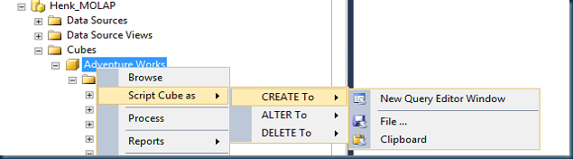
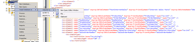
To get to all data type information just ‘right click’ on the SSAS Database name and script the entire DB into a new query Editor Window.
Search through the xml for the query source name that is used for the partition, like: msprop:DbTableName="FactInternetSales"

These should match the SQL Server data types; check especially for unsignedByte, short, String lengths and Doubles (slow) vs floats (fast). (We do have to warn you about the difference between an exact data type like Double vs an approximate like Float here).
A link to a list of how to map the Data types is available here.
How can we quickly check and align the data types best because to go over them all manually one by one isn’t funny as you probably just found out. By searching the net I ran into a really nice and useful utility written by John Tunnicliffe called ‘CheckCubeDataTypes’ that does the job for us; it compares a cube’s data source view with the data types/sizes of the corresponding dimensional attribute. (Kudos John!) But unfortunately even after making sure the datatypes are aligned and running Kernrate again shows that DataConvert is still the number one consumer of CPU ticks on the SSAS side.
3) Optimize the data types at the source
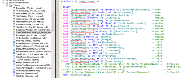
To proof that this conversion is our next bottleneck we can also create a view on the database source side and explicitly cast all fields to make sure they match the cube definition. (This will also be an option to test environments where you don’t own the cube source & databases)
Maybe as best-practice CAST all columns even if you think the data types are right and exclude also the ones that are not used for processing the Measure group from the View. (For example, to process the FactInternetSales Measure Group from the AdventureWorks2012 DW cube we don’t need [CarrierTrackingNumber], [SalesOrderNumber], [PromotionKey] and [CustomerPONumber]) ; every bit that we don’t have push over the wire and process from the database source is a pure win. Just create a view with the name ‘Speed’ like to give it a try.

(Note: always be careful when changing data types!
For example, in the picture above, using the ‘Money’ data type is Okay because it is used for FactInternetSales, but Money is not a replacement for all Decimals (as it will only keep 4 digits behind the decimal point and doesn’t provide the same range) so be careful when casting data types and double check you don’t lose any data!)
Result: by using the data type optimized Speed view as source the total throughput increased from 5 to 6.6-6.8 Million rows Read/sec and 4600% CPU usage (== 147K rows/CPU). That’s 36% faster. We’re getting there!
The picture also shows that one of the physical CPU sockets (look at the 2nd line of 16 cores in Numa Node 1) is completely max’d out:

4) Create a ‘Static Speed’ View for testing
If you would like to take the database performance out of the equation something I found useful is to create a static view in the database with all the values pre-populated this way there will still be a few logical reads from the database but significant less physical IO.
Approach:
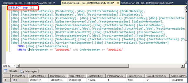
1) Copy the original query from the cube:

2) Request just the SELECT TOP (1):
 From...")
3) Create a Static view:
Add these values to a view named ‘Static_Speed’ and cast them all:

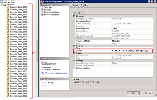
4) Create an additional test partition that queries the new Static_view

5) Copy this test partition multiple times
Create at least as many test partitions equal to the number of cores in your server, or more:
Script the test partition as created in step 4):

Create multiple new partitions from it by just changing the <ID> and <Name> ; these will run the same query using just the static view. This way you can test the impact of your modifications to the view quickly and at scale!
6) Processing the test partitions
Process all these newly created test partitions who will only query the statics view and select as many of them or more as the number of CPU’s you have available in your SSAS server.
Determine the maximum processing capacity of your cube server
by monitoring the ‘Rows Read/sec’!
Wrap Up
If you have a spare moment to check out the workload performance counters of your most demanding cube servers you may find that there is room for improvement. If you see flat lines during the Cube processing I hope your eyes will now start to blink; by increasing the number of connections or checking if you don’t spend your CPU cycles on data type conversions you may get a similar of over 3x improvement, like shown in the example above. By looking at the Task Manager CPU utilization where just one of the NUMA nodes is completely max’d out might indicate its time to start looking into some of the msmdsrv.ini file settings…

 , maxing out a single CPU.")


